Nuklei was initially designed to model density functions defined on the Special Euclidean group \( SE(3) \) (or on a subspace thereof). This page reviews the theory behind density estimation and density integrals particularized to \( SE(3) \) data. This is the place to start if you haven't yet heard of nonparametric representations, quaternions, or von Mises-Fisher distributions. Once you feel comfortable with the material presented here (feel free to explore the references given below!), move on to Kernels, kernel density estimation, kernel regression, which explains which concepts Nuklei implements, and how they are implemented. Keep in mind that the Nuklei implementation doesn't strictly follow the text presented on this page. For instance, in the text below, 3D positions are modeled with Gaussian distributions. Nuklei, on the other hand, offers both Gaussian and triangular kernels for modeling positions, and triangular kernels are used by default in kernel density estimation and kernel logistic regression. More...

Nuklei was initially designed to model density functions defined on the Special Euclidean group \( SE(3) \) (or on a subspace thereof). This page reviews the theory behind density estimation and density integrals particularized to \( SE(3) \) data. This is the place to start if you haven't yet heard of nonparametric representations, quaternions, or von Mises-Fisher distributions. Once you feel comfortable with the material presented here (feel free to explore the references given below!), move on to Kernels, kernel density estimation, kernel regression, which explains which concepts Nuklei implements, and how they are implemented. Keep in mind that the Nuklei implementation doesn't strictly follow the text presented on this page. For instance, in the text below, 3D positions are modeled with Gaussian distributions. Nuklei, on the other hand, offers both Gaussian and triangular kernels for modeling positions, and triangular kernels are used by default in kernel density estimation and kernel logistic regression.

Parametrization

This page reviews kernel methods for data defined on the following domains:

The group of 6D poses. A 6D pose, also referred to as transformation, is composed of a 3D position and a 3D orientation . The group of 6D poses is referred to as the Special Euclidean group. It is denoted by
\[ SE(3) = \mathbb R^3 \times SO(3), \]
where \(SO(3)\) is the group of 3D rotations, and \( \times \) denotes a semidirect product. Poses are parametrized by a pair composed of a 3D position and a 3D orientation. Orientations can be parametrized in multiple ways, e.g., with rotation matrices, Euler angles, or unit quaternions. We parametrize 3DOF orientations with unit quaternions. Unit quaternions form the 3-sphere \( S^3 \) (the set of unit vectors in \( \mathbb R^4 \)). A rotation of \( \alpha \) radians about a unit vector \( v = (v_x, v_y, v_z) \) is parametrized by a quaternion \( q \) defined as
\[ q = \left(\cos\frac\alpha 2, v_x\sin\frac\alpha 2, v_y\sin\frac\alpha 2, v_z\sin\frac\alpha 2 \right). \]
Because a rotation of \( \alpha \) radians about \( v \) is equivalent to a rotation of \( -\alpha \) about \( -v \), \( q \) and \( -q \) correspond to the same rotation. Consequently, unit quaternions form a double cover of \( SO(3) \) — every rotation exactly corresponds to two unit quaternions. Quaternions offer a clear formalism for the definition of position-orientation densities (see below). From a numerical viewpoint, they are stable and free of singularities. Finally, unit quaternions allow for the definition of a rotation metric that roughly reflects our intuitive notion of a distance between rotations. The distance between two rotations \( \theta \) and \( \theta' \) is defined as the angle of the 3D rotation that maps \( \theta \) onto \( \theta' \). This metric can be easily and efficiently computed using unit quaternions as twice the shortest path between \( \theta \) and \( \theta' \) on the \( 3 \)—sphere,
\[ \textrm{d}\left(\theta, \theta'\right) = 2\arccos\left|\theta ^\top \theta'\right|, \]
where \( \theta^\top \theta' \) is the inner (dot) product of \( \theta \) and \( \theta' \). In this expression, we take the absolute value \( |\theta ^\top \theta'| \) to take into account the double cover issue mentioned above.
The space of the pairs composed of a 3DOF position and an axial 2DOF orientation (a line orientation in 3D). Axial 2DOF orientations are parametrized with 3D unit vectors. We note that unit vectors form a double cover of axial 2DOF orientations, as an orientation \(v\) is equivalent to \( -v \). The space of the pairs composed of a 3DOF position and an axial 2DOF orientation is denoted by
\[\mathbb R^3 \times S^2. \]

Nonparametric Density Estimation

Density estimation generally refers to the problem of estimating the value of a density function from a set of random samples drawn from it. Density estimation methods can loosely be divided into two classes: parametric or nonparametric. Parametric methods model a density with a set of heavily parametrized kernels. The number of kernels is generally smaller than the number density samples available for computing the model. The price to pay for the smaller number of kernels is the substantial effort required to tune their parameters. The most famous parametric model is the Gaussian mixture, which is generally constructed by tuning the mean and covariance matrix of each Gaussian kernel with the Expectation-Maximization algorithm.

Nonparametric methods represent a density simply with the samples drawn from it. The probabilistic density in a region of space is given by the local density of the samples in that region. A density can be estimated by simple methods such as histograms, or more sophisticated methods like kernel density estimation. Kernel density estimation (KDE) works by assigning a kernel function to each observation; the density is computed by summing all kernels. By contrast to parametric methods, these kernels are relatively simple, generally involving a single parameter defining an isotropic variance. Hence, compared to classical parametric methods, KDE uses a larger number of simpler kernels.

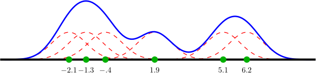Kernel estimation (blue) of a density observed through 6 samples (green). The dashed red lines illustrate the gaussian kernels associated to each sample. The estimate is obtained by summing all kernels. To form a proper density, the function represented by the blue line should be normalized by dividing it by 6.

In this work, densities are modeled nonparametrically with KDE. This choice is primarily motivated by the structure of the position—orientation domains on which they are defined: Capturing pertinent position-orientation correlations within a single parametric function is very complex, while these correlations can easily be captured by a large number of simple kernels. Also, the nonparametric approach eliminates problems like mixture fitting, choosing a number of components, or having to make assumptions concerning density shape (e.g. normality).

A density \( d(x) \) is encoded by a set of observations \( \hat x_{i} \) drawn from it, which we will refer to as particles. Density values are estimated with KDE, by representing the contribution of the \( i^\textrm{th} \) particle with a local kernel function \( \mathcal K\left(\cdot ; \hat x_i, \sigma\right) \) centered on \( \hat x_i \). The kernel function is generally symmetric with respect to its center point; the amplitude of its spread around the center point is controlled by a bandwidth parameter \( \sigma \). For conciseness, particles are often weighted, which allows one to denote, e.g., a pair of identical particles by a single particle of double mass. In the following, the weight associated to a particle \( \hat x_{i} \) is denoted by \( w_{i} \).

KDE estimates the value of a continuous density \( d \) at an arbitrary point \( x \) as the weighted sum of the evaluation of all kernels at \( x \), i.e.,

\[ d(x) \simeq \sum_{i=1}^n w_i \mathcal K\left(x ; \hat x_i, \sigma\right), \]

where \( n \) is the number of particles encoding \( d \). Random variates from the density are generated as follows:

First, a particle \( \hat x_i \) is selected by drawing \( i \) from
\[ P(i = \ell) \propto w_{\ell}. \]
(This effectively gives a higher chance to particles with a larger weight.)
Then, a random variate \( x \) is generated by sampling from the kernel \( \mathcal K\left(x ; \hat x_i, \sigma\right) \) associated to \( \hat x_i \).

Defining Densities on ( SE(3) )

In order to define densities on \( SE(3) \), a position-orientation kernel is required. We denote the separation of kernel parameters into position and orientation by

\begin{align} x = (\lambda, \theta)&\qquad x\in SE(3),\quad \lambda\in\mathbb R^3,\quad \theta\in SO(3),\\ \mu = (\mu_t, \mu_r)&\qquad \mu \in SE(3),\quad \mu_t \in \mathbb R^3,\quad \mu_r \in SO(3),\\ \sigma = (\sigma_t, \sigma_r)&\qquad \sigma_t, \sigma_r \in\mathbb R_+. \end{align}

The kernel we use is defined with

\[ \mathcal K\left(x ; \mu, \sigma\right) = \mathcal L\left(\lambda ; \mu_t, \sigma_t\right) \mathcal O_4\left(\theta ; \mu_r, \sigma_r\right), \]

where \( \mu \) is the kernel mean point, \( \sigma \) is the kernel bandwidth, \( \mathcal L \) is an isotropic location kernel defined on \( \mathbb R^3 \), and \( \mathcal O_4 \) is an isotropic orientation kernel defined on \( SO(3) \).

For \( \mathbb R^3 \), we can simply use a trivariate isotropic Gaussian kernel

\[ \mathcal L\left(\lambda; \mu_t, \Sigma_t\right) = C_g(\Sigma_t) e^{-\frac{1}{2}( \lambda - \mu_t)^\top \Sigma_t^{-1} (\lambda - \mu_t)}, \]

where \( C_g(\cdot) \) is a normalizing factor and \( \Sigma_t = \sigma_t^2 \mathbf{I} \). The definition of the orientation kernel \( \mathcal O_4 \) is based on the von Mises—Fisher distribution on the 3-sphere in \( \mathbb R^4 \). The von Mises—Fisher distribution is a Gaussian-like distribution on \( S^3 \). It is defined as

\[ \mathcal F_4\left(\theta ; \mu_r, \sigma_r\right) = C_4(\sigma_r)e^{\sigma_r \; \mu_r^T \theta}, \]

where \( C_4(\sigma_r) \) is a normalizing factor, \( \theta \) and \( \mu_r \) are unit quaternions, and \( \mu_r^T \theta \) is a dot product. Because unit quaternions form a double cover of the rotation group, \( \mathcal O_4 \) has to verify \( \mathcal O_4\left(q ; \mu_r, \sigma_r\right) = \mathcal O_4\left(-q ; \mu_r, \sigma_r\right) \) for all unit quaternions \( q \). We thus define \( \mathcal O_4 \) as a pair of antipodal von Mises—Fisher distributions,

\[ \mathcal O_4\left(\theta ; \mu_r, \sigma_r\right) = \frac {\mathcal F_4\left( \theta ; \mu_r, \sigma_r \right) + \mathcal F_4 \left(\theta; -\mu_r, \sigma_r\right)}2. \]

We note that the von Mises—Fisher distribution involves the same dot product as the rotation metric defined above ( \( \textrm{d}\left(\theta, \theta'\right) = 2\arccos\left|\theta ^\top \theta'\right| \)). The dot product \( \mu_r^\top \theta \) is equal to \( 1 \) when \( \mu_r = \theta \). The dot product decreases as \( \theta \) moves further away from \( \mu_r \), to reach \( 0 \) when \( \theta \) is a \( 180^\circ \) rotation away from \( \mu_r \). In this range of values, the von Mises—Fisher kernel thus varies between \( C_4(\sigma_r)e^{\sigma_r} \) and \( C_4(\sigma_r) \). While \( e^{\sigma_r} \) grows rapidly with \( \sigma_r \), \( C_4(\sigma_r) \) rapidly becomes very small. This makes the computation of \( \mathcal F_4 \) numerically difficult. A robust approximation of \( \mathcal F_4 \) can be obtained with

\[ \mathcal F_4 \left(\theta ; \mu_r, \sigma_r\right) \simeq e^{\sigma_r \; \mu_r^T \theta + C'_4(\sigma_r)}, \]

where \( C'_4(\sigma_r) \) approximates the logarithm of \( C_4(\sigma_r) \)(Abramowitz 1965, Elkan 2006). However, since \( \sigma_r \) is common to all kernels forming a density, using

\[ \mathcal{\tilde F_4} \left(\theta ; \mu_r, \sigma_r\right) = e^{- \sigma_r\left(1-\mu_r^T \theta\right)} \]

instead of \( \mathcal{F_4} \) in the expression of \( \mathcal O_4 \) above will yield density estimates equal to \( d \) (defined above) up to a multiplicative factor, while allowing for efficient and robust numerical computation. This alternative will be preferred in all situations where \( d \) need not integrate to one.

Defining Densities on ( \mathbb R^3\times S^2 )

Turning to densities defined on \( \mathbb R^3\times S^2 \), let us define

\begin{align} x = (\lambda, \theta)&\qquad x\in \mathbb R^3\times S^2, \quad \lambda\in\mathbb R^3, \quad \theta\in S^2,\\ \mu = (\mu_t, \mu_r)&\qquad \mu \in \mathbb R^3\times S^2,\quad \mu_t \in \mathbb R^3,\quad \mu_r \in S^2,\\ \sigma = (\sigma_t, \sigma_r)&\qquad \sigma_t, \sigma_r \in\mathbb R_+. \end{align}

The \( \mathbb R^3\times S^2 \) kernel is defined as

\[ \mathcal K_3\left(x ;\mu, \sigma \right) = \mathcal N\left(\lambda ; \mu_t, \sigma_t\right) \mathcal O_3\left(\theta ; \mu_r, \sigma_r\right), \]

where \( \mathcal{O_3} \) is a mixture of two antipodal \( S^2 \) von Mises—Fisher distributions, i.e.,

\begin{align} \mathcal O_3\left(\theta ; \mu_r, \sigma_r\right) &= \frac {\mathcal F_3\left(\theta ; \mu_r, \sigma_r \right) + \mathcal F_3\left(\theta ; -\mu_r, \sigma_r\right) }2,\\ \mathcal F_3\left(\theta ; \mu_r, \sigma_r\right) &= C_3(\sigma_r)e^{\sigma_r \; \mu_r^T \theta}. \end{align}

In the expression above, \( C_3(\sigma_r) \) is a normalizing factor, which can be written as

\[ \frac{\sigma_r}{2\pi\left(e^\sigma_r-e^{-\sigma_r}\right)}. \]

\( \mathcal{F_3} \) can thus be written as

\[ \mathcal F_3\left(\theta ; \mu_r, \sigma_r\right) = \frac{\sigma_r}{2\pi\left(1-e^{-2\sigma_r}\right)} e^{-\sigma_r\left(1-\mu_r^T\theta\right)}, \]

which is easy to numerically evaluate. As for \( SE(3) \) densities, when \( d \) need not integrate to one, the normalizing constant can be ignored.

Evaluation and Simulation

As the kernels \( \mathcal{K} \) and \( \mathcal{K_3} \) factorize to position and orientation factors, they are simulated by drawing samples from their position and orientation components independently. Efficient simulation methods are available for both normal distributions and von Mises—Fisher distributions.

From an algorithmic viewpoint, density evaluation is linear in the number of particles \( n \) supporting the density. Asymptotically logarithmic evaluation can theoretically be achieved with \( kd \)-trees and slightly modified kernels: Considering for instance \( SE(3) \) densities and the notation introduced above, let us define a truncated kernel \( \mathcal{K'} \) as

\[ \mathcal K'\left(x ; \mu, \sigma\right) = \begin{cases} \mathcal K\left(x ; \mu, \sigma\right) &\textrm{ if } \textrm{d}\left(\lambda, \mu_t\right) < \lambda_\ell \textrm{ and } \textrm{d}\left(\theta, \mu_r\right) < \theta_\ell,\\ 0 &\textrm{ else,} \end{cases} \]

where \( \lambda_\ell \) and \( \theta_\ell \) are fixed position and orientation thresholds. The value at \( \left(\lambda, \theta\right) \) of a density modeled with \( \mathcal{K'} \) only depends on particles whose distance to \( \left(\lambda, \theta\right) \) is smaller than \( \lambda_\ell \) in the position domain, and smaller than \( \theta_\ell \) in the orientation domain. These particles can theoretically be accessed in near-logarithmic time with a \( kd \)-tree.

However, traversing a \( kd \)-tree is computationally more expensive than traversing a sequence. Hence, \( kd \)-trees only become profitable for \( n \) larger than a certain threshold. In the case of our 5DOF or 6DOF domains and sets of \( 500 \)— \( 2000 \) particles, we have observed best performances when organizing particle positions in a \( kd \)-tree, while keeping orientations unstructured. Density evaluation is always sub-linear in the number of particles, and it approaches a logarithmic behavior as \( n \) increases.

Resampling

In the next chapters, certain operations on densities will yield very large particle sets. When the number of particles supporting a density becomes prohibitively high, a sample set of \( n \) elements will be drawn and replace the original representation. This process will be referred to as resampling. For efficient implementation, systematic sampling can be used to select \( n \) kernels from

\[ P(i = \ell) \propto w_{\ell}. \]

In the following, \( n \) will generally denote the number of particles per density.

Integration

The models presented in the next chapters make extensive use of approximate integration of density functions. In this work, approximate integration is generally carried out through Monte Carlo integration, which is briefly introduced below. The remainder of the section then details the convolution of \( SE(3) \) and \( \mathbb R^3\times S^2 \) densities, as this operation is instrumental in the models of the next chapters.

Monte Carlo Integration

Integrals over \( SE(3) \) and \( \mathbb R^3\times S^2 \) are solved numerically with Monte Carlo methods. Monte Carlo integration is based on random exploration of the integration domain. By contrast to classical numerical integration algorithms that consider integrand values at points defined by a rigid grid, Monte Carlo integration explores the integration domain randomly.

Integrating the product of two density functions \( f(x) \) and \( g(x) \) defined on the same domain is performed by drawing random variates from \( g \) and averaging the values of \( f \) at these points

\[ \int f(x)g(x) \textrm{d} x \simeq \frac 1n \sum_{i=1}^n f(x_i) \quad \textrm{where} \quad x_i \sim g(x). \]

Cross-Correlation

Let \( f \) and \( g \) be two density functions with domain \( D \), where \( D \) is either \( SE(3) \) or \( \mathbb R^3\times S^2 \). Let also

\[ t_x(y) : D\rightarrow D \]

denote the rigid transformation of \( y \) by \( x \), with \( y\in D \) and \( x\in SE(3) \). The \( SE(3) \) cross-correlation of \( f \) and \( g \) is written as

\[ c(x) = \int f\left(y\right) g(t_{x}\left(y\right)) \mathrm{d}y. \]

As both \( f \) and \( g \) have unit integrals, Fubini's theorem guarantees that \( c \) also integrates to one.

The cross-correlation of \( f \) and \( g \) is approximated with Monte Carlo integration as

\[ c(x) \simeq \frac 1n \sum_{\ell=1}^n g(t_{x}(y_\ell)) \quad \textrm{where} \quad y_\ell \sim f(y). \]

Sampling from \( c(x) \) can be achieved by simulating \( h(x) = g(t_{x}(y_f)) \), where \( y_f\sim f(y) \). The simulation of \( h(x) \) depends on the domain \( D \) on which \( f \) and \( g \) are defined. We first consider the case \( D = SE(3) \). In this case, drawing a sample from \( h(x) \) amounts to computing the (unique) transformation \( x_* \) that maps \( y_f \) onto \( y_g \), where \( y_g\sim g(y) \). When \( D = R^3\times S^2 \), the transformation between \( y_f \) and \( y_g \) is not unique anymore; sampling \( h(x) \) is done by selecting one transformation from a uniform distribution on the transformations that map \( y_f \) onto \( y_g \).